Calculating the Spectra of Helium
This article describes how to use simple Rydberg-like formulas to
accurately calculate both the spectral lines and line intensities. The
calculation of the spectra for atoms other than hydrogen or hydrogen
like ions has long been considered to be complex multi-body problem
which can only be solved with the use of supercomputers. Calculating
the line intensities does not appear to be addressed at all in the
existing literature. However, if you create a simple graph of the line
frequencies and intensities for Helium, a striking and predictable
pattern appears which suggests that the spectra and the intensity can
be calculated using simple formulas based on the Rydberg formula. This
pattern also appears in lithium and beryllium.
The list of spectral data can be found at:
http://physics.nist.gov/
A description of the Rydberg forumula can be found at:
http://en.wikipedia.org/wiki/
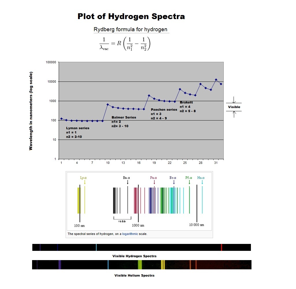
The Rydberg formula can be used to calculate the atomic spectra of
Hydrogen. Plotting the spectra on a log scale reveals a staircase pattern
http://franklinhu.com/hydrogenspectra.jpg
It can be extended to calculate the spectra of Hydrogen-
like ions by adding a factor of Z^2. These ions are any atoms which
have been fully ionized and a single electron interacts with only the
positively charged nucleus. For example, if you remove the 2 electrons
from Helium, this ion is identified as He II. If you only remove 1
electron, this is called He I. The spectra for He II can be calculated
using only the extended Rydberg formula.
If you plot the calculated He II spectra wavelength against the
electron level transitions (e.g. 1->2, 1->3, ... 2->3, 2->4..etc.) on
a logarithmic scale, the graph appears like a staircase leading up.
When the starting energy level increase by 1 (e.g 1->2 vs. 2->3), this
causes a large step up in the frequency. The calculated spectra
matches up well with the observed He II spectra.
Using the data from the NIST database and plotting spectral lines for
He II against the observed values for He I, the plot for He I also
appears as this same staircase pattern, but at a longer wavelength.
This nearly identical shape suggests that the He I spectra can be
calculated as simply being a scaled version of the He II spectra.
The graph of He II (shown in pink) and He I (shown in yellow) spectra
values can be found at:
http://franklinhu.com/
The Excel spreadsheet used to create this graph and a Microsoft word
document of this article is avaliable upon request.
The NIST data contains the electronic transitions and the ions that
represent the observed wavelength. In most cases, this is what was
used to plot the point on the graph. The Y axis shows the wavelength
in nanometers. The X axis lists the 32 electron transitions in
ascending order.
Since the He I spectrum appears so close to the He II spectrum, is
there a simple formula that can transform one into the other? This is
basically a curve fitting exercise. It does appear that a different
formula can be applied at each energy level to calculate the spectral
wavelengths.
For N1 = 1 (transitions starting at N1 = 1), the curve can be
represented by the formula:
Rydberg(N1,N2)+28.14-(N2)*0.
Where Rydberg(N1,N2) represents the result of the extended Rydberg
formula for He II and N1 represents the starting electron level and N2
represents the ending electron level. For example, the 1->2 transition
calculates to 58.427 nm and matches with the observed result of 58.43
nm. This appears to be a constant minus a scaling factor based on N2.
For N1 = 2, the formula changes to:
Rydberg(1,N2)*13-N2*3.55
This appears to be a scaling factor on the Rydberg formula minus a
scaling factor of N2, howevever, the shape of the curve better matches
N1=1, so the Rydberg formula is shown with a starting level N1=1.
For n = 3,4,5,6 the formula is:
Rydberg(N1,N2)*4
This is a straight scaling by 4 for all of the higher energy level
shells.
The following is the calculated He I spectral data. Columns N1 & N2
represent the electron shell transition number. The third column
represents the observed wavelength and fourth represents the
calculated wavelength. The last column shows the difference between
the observed and calculated values which is typically less than a
percent difference. On the graph, you will see observed wavelengths
plotted in blue behind the yellow calculated values. The values are so
close, that you can barely see the differences between the two.
N1 N2 Observe Calc % Difference
1 2 58.43 58.43 0.00
1 3 53.70 53.64 0.12
1 4 52.22 52.26 0.09
1 5 51.56 51.65 0.18
1 6 51.20 51.31 0.21
1 7 50.99 51.09 0.19
1 8 50.86 50.93 0.14
1 9 50.77 50.81 0.08
1 10 50.70 50.71 0.02
2 3 388.87 387.78 0.28
2 4 318.77 322.53 1.17
2 5 294.51 301.71 2.38
2 6 282.91 290.75 2.70
2 7 276.38 283.32 2.45
2 8 272.32 277.48 1.86
2 9 269.61 272.46 1.05
2 10 267.71 267.91 0.08
3 4 1868.53 1874.61 0.32
3 5 1279.06 1281.47 0.19
3 6 1031.12 1093.52 5.71
3 7 970.26 1004.67 3.43
3 8 960.34 954.35 0.63
3 9 952.62 922.66 3.25
4 5 4048.99 4050.08 0.03
4 6 3091.69 2624.45 17.80
4 7 2113.78 2164.95 2.36
4 8 1954.31 1944.04 0.53
5 6 7455.82
5 7 4651.26
5 8 3738.53
6 7 12365.19
6 8 7498.43
These calculations do not account for all of the 96 observed He I
spectral lines. This limited calculation provides at most 32 values
and for He I, there are no observed values for transitions starting
from the 5 & 6 level, so this calculation accounts for 27 or 96 lines.
There may certainly be other processes involved which create the other
observed values, however, it is remarkable how closely the observed
values can be matched with the calculated ones.
Another aspect of atomic spectra which appears to be absent in the
literature is the calculation of the relative intensity for the
spectral lines. If you do a similar plot of energy level transitions
against the relative intensity found in the NIST data for hydrogen,
this produces a very regular saw tooth shape. This is shown in the
following graph for Hydrogen in pink.
http://franklinhu.com/
The relative intensity can be calculated for N1=1,2,3 as:
(1/N1^3*1000)*1/(N2-N1)^(2.23-
For N1 = 4,5,6
(1/N1^3*1000)*1/(N2-N1)
The intensity appears to drop as the inverse cube. These calculations
are able to reproduce the observed relative intensities as found in
the NIST data. The Hydrogen graph shows the calculated values in
yellow and the observed values in pink.
This exact same formula also appears to apply to the relative
intensity for He II. The graph for Helium shows the experimentally
observed values in light blue and the calculated values in purple for
He II. For He I, the intensity follows the formula for N1=1, it
partially follows when N1=2, but after that the relative intensity
becomes chaotic and does not appear to follow any pattern.
The same spectra analysis can be applied to the next element in the
periodic table which is lithium. The graph of the lithium spectra can
be found at:
http://franklinhu.com/
The calculated extended Rydberg formula spectra for Li III is shown in
blue.
For lithium II and I, the electron transition states stated in the
NIST data do not directly provide all of the transition states
required to plot the points on this graph. In this case, some of the
points have been selected based upon where one would "predict" where a
point would exist on the graph and using those points having the
greatest relative intensity. The regularity of the pattern allows you
to make these predictions. If you take a ruler and match up with any 2
of the peaks of the steps, you can predict where the next step should
appear. After this peak, one would expect to find a set of 1/N2^2
decreasing values and relative intensities. By using this methodology,
the experimental data has been matched to the electron transitions as
shown in pink in the graph.
The Li II values (shown as yellow in the graph) can be calculated with
the following formulas:
For N1=1
Rydberg(N1,N2)+6.42
For N1=2
Rydberg(N1,N2)*2
For N1=3,4,6
Rydberg(N1,N2)*2.3
For N1=5
Rydberg(N1,N2)*2.145+(N2-5)*
Spectral data points can also be found for Li I which has 3 electrons
bound to the atom with only 1 free electron. This also shows the
familiar staircase pattern. The formulas for Li I have not been
calculated, but it should be obvious that a best fit formula could be
found for these data points.
The calculations match fairly closely with the observed Li data except
for N1=1 and N2=5-9. Here we see an unusual dip in the wavelength
compared to calculations. This dip can also be seen in the Li I data
as well, so there may be somethIng structural in Li that causes this
deviation.
The analysis for the next element Beryllium becomes even more
difficult as we are faced with a nearly continuous spectra. For
example, to do the analysis of Be I, the only points that appeared to
be known with any confidence are the very highest transitions which
have very few spectral lines in the longest wavelengths. Based on the
slope of those data points, the rest of the points were selected. For
Be, even the ion identification needed to be occasionally ignored to
find best fit data points. Due to this difficulty, the exact quality
of the data point selection is questionable. However, there is enough
data to speculate that the overall shape and slope of the graph is
correct and the graph contains most of the brightest observed lines.
The graph of Beryllium can be found at:
http://franklinhu.com/
Compared with lithium, we see that the Li III and Li II are closely
spaced like Be IV and Be III. The next ion Li I and Be II appear to be
further spaced away. Be I appears closely spaced with Be II. This
similar pattern suggests that the ions may follow a predictable energy
pattern and it provides confidence that the Be graph correctly
describes the energy pattern.
Conclusion:
From the spectral data for hydrogen through beryllium, a regular
pattern can be seen in the data. The spectra may initially appear to
be a random collection of oddly spaced lines, but when you look at the
pattern of overlapping wavelengths created by the different ions, it
is easy to see how such a pattern is created.
A relatively crude curve matching formula was created to match this
pattern which was based only upon the starting and ending electron
level N1 & N2. It is possible that more sophisticated analysis will
reveal an even simpler formula to describe the very regular staircase
pattern found in the data.
Since the spectra can be described entirely as a function of N1 & N2,
it would appear that the problem of calculating spectra may not be a
complex multi-body problem as was previously thought. Whatever effect
that the electrons have in shielding the nucleus, this effect appears
to be constant and so you only need to consider the nucleus and the
electron as a simple two body problem like it is in the original
Rydberg formula.
However, not all of the spectra can be explained, as there are still
numerous unexplained lines. However, by eliminating the points which
can be explained, it may be possible to find further patterns in the
unexplained lines. These other lines may require complex multi-body
calculations. These calculations also do not take into account any
fine differences such as the lamb shift. It only covers transitions
that can be described using N1 and N2 as parameters.
Only the first four elements have been examined using this analysis.
This can be extended to the other elements as well and other
regularities may appear which may further enhance our understanding of
the atom. The formulas derived could also have other uses such as in
the generation of synthetic spectra for use in astronomy and may lead
to a more accurate understanding of which lines belong to what
electronic transition. These formulas may allow the prediction and
detection of as of yet undiscovered spectral lines.
It is extremely surprising that the regularity of the spectral lines
has not been prominently noted in the literature. The analysis done
here is extremely simple and obvious. The regularity of the H and He
II relative spectral intensity should be part of any standard
description of the spectra for H and He as it follows a very regular
pattern.
The formulas presented may have been created Ad Hoc to match the data
and it is unclear why they have the form that they do. However, like
Bohr and Rydberg who were also unable to explain why the spectra
appear the way they do, it is important to continue to explore and
find patterns within the data that can be described by simple formulas
in the hopes that one will find the underlying mechanisms. This
analysis deserves further research and may open new avenues in the
science of the atom.